12/08/2014
Abstract
Salamanders provide important ecosystem services and are essential to maintaining a healthy ecosystem, at least in the Northern Hemisphere. More than a third of all amphibian species are threatened or already extinct, and their decline is being monitored closely. Accurate estimates of the area each species occupies an important measure when evaluating a species conservation status. Conservation groups make decisions based on these calculations of area, but often times wrongly use extent of occurrence rather than the area of occupancy. This is largely due to the lack of area of occupancy distribution maps in science. Salamanders are secretive creatures and spend most of their lives burrowed under logs and rocks in a singular land cover type: forests. Extent of occurrence maps fail to take land cover into account and include obvious areas of unsuitable, making calculation of area extrapolated from these maps meaningless. In response to the absence of area of occupancy map shapefiles available on the web for Pennsylvania’s salamanders, I elected to map six of them. In addition to mapping the area of occupancy, I also made distribution maps of the extent of occurrence type for comparison.
Introduction
Salamanders are of the order Caudada and include 10 families, 24 genera, and more than 600 species. The evolution of salamanders’ dates back to the Middle Jurassic, and the oldest known salamander fossil is estimated to be 161 million years old (myr). During this time, the super continent Pangea was splitting into two primary landmasses. As it turns out, salamander species are restricted in their distribution to the United States, Canada and Asia. From a biogeography standpoint, this would mean that salamanders evolved on Laurasia sometime after this split of Pangea. Laurasia today can be considered the northern hemisphere and includes Asia, the United States, and Canada. Gondwana, the landmass making South America, Africa, and Australia, lacks salamanders. This finding is consistent with the estimated time the two land masses split, which is believed to have occurred around 150 myr ago. These animals are some of the few still roaming the earth today that existed with dinosaurs. Their importance to forest ecosystems in the northern hemisphere is unmatched.
Maintaining arthropod populations, serving as prey for animals on higher trophic levels, and reducing carbon on the forest floor are just a few of the important ecosystem services salamanders provide. Because salamanders absorb water, oxygen, and other gases through their skin, they are the first to be negatively impacted by pollution and other environmental changes. This characteristic makes them important indicators of ecosystem health and biodiversity.
Interest in amphibian health and conservation has grown rapidly in the last decade largely due to their decline. Today, more than a third of all amphibian species are threatened or have already gone extinct. The decline in amphibian populations is well documented in frog populations, but has yet to be well-documented in salamanders. Conservation groups such as the International Union for Conservation of Nature (IUCN) Red List actively assess the health of salamander species, listing half of the world’s salamanders as threatened. If a species is threatened, it means that the extant or surviving populations are either critically endangered, endangered, or considered vulnerable. For a species to be classified as threatened, it has to meet at least one of the criterion making a species at risk for extinction. These criteria range from severe fragmentation to a reduction in the number of mature individuals. One of the strongest indicators for animal population health is that of its habitat. What is the area this species occupies, and has it declined? Questions such as these are easy to calculate using a geographic information system (GIS) provided there are accurate distribution maps created.
In the science of distribution mapping, there are two primary types. These include the extent of occurrence and the area of occupancy. The extent of occurrence distribution maps represent the shortest contiguous area for all known occurrences of the species. Extent of occurrence maps include large areas of clearly unsuitable habitat. Because these maps do not incorporate important environmental variables into their construction, values of area calculated from these polygons cannot be considered actual estimates. Area of occupancy maps on the other hand do take land cover and other ecosystem requirements into account, representing the smallest area required for the survival of existing populations. Values of area calculated from these maps do hold meaningful and should be used to guide conservationists. I was therefore disconcerted to discover that the maps featured on the IUCN Red List website were of the extent of occurrence type rather than area of occupancy. This tells me that there is a need for more accurate distribution maps for salamander species.
In the following analysis, I am working to create area of occupancy maps, with meaningful calculations of area, for six of Pennsylvania’s salamanders. In addition, I use two different methods to construct extent of occurrence maps for each species. The species mapped span across four genera and include the Jefferson’s Salamander (Ambystoma jeffersonianum), the Yellow-Spotted Salamander (Ambystoma maculatum), the Marbled Salamander (Ambystoma opacum), the Eastern Hellbender (Cryptobranchus alleganiensis), the Longtail Salamander (Eurycea longicauda), and the Eastern Redbacked Salamander (Plethodon cinereus).
Data and Methods
Data required to construct these distribution maps included administrative boundaries at the county level, which I downloaded from the US Census Bureau website, the National Land Cover Dataset from 2011, and a text-encoded list of X, Y occurrences. The text encoded list of occurrences were downloaded from the Global Biodiversity Information Facility (GBIF) database. The data required minor cleaning such as relabeling attribute fields and removing data attributes which were irrelevant to our analyses. The GBIF database is free and open, including more than 500 million occurrences from hundreds of sources including museum records, private collections, and citizen science platforms such as iNaturalist. Citizen science data requires zero resources to produce on the part of the science community, making it an invaluable source of information.
Because the validity of my distribution maps rely on the observations to be accurate, I chose to study six species of Pennsylvania’s salamanders that I felt were the easily identifiable. Morphological characteristics used by herpetologists to distinguish between species include snout length, body size, patterning and coloration, and the number of toes and costal grooves. The only characteristics I felt comfortable assuming non-experts will understand and be able to accurately characterize was coloration and body size. The yellow-spotted salamander, for instance, is pitch black with bright yellow spots. The Eastern Red-backed salamander on the other hand features a heavily speckled black and white belly and a bright colored dorsal stripe that runs the length of its body. The eastern hellbender salamander, while gray, is a giant salamander which can reach up to two feet in length! In short, each of the six species mapped were extremely distinctive in appearance. Photographs of each are shown in Figure 1.
I wanted to create extent of occurrence maps for each salamander species. The purpose of making extent of occurrence maps myself, when they are available for download online for free, was so that I can compare calculations of area from distribution maps created using the same datasets. The IUCN does not release detailed metadata detailing the sources and methodology used for creating the distribution map shapefiles featured on their website. By definition, the extent of occurrence is the area contained within the smallest contiguous area encompassing all known locations for where a species is known to occur. In other words, the extent of occurrence is a convex polygon which wraps around all documented locations.
To begin, I reprojected all of my data layers to be in a projected coordinate system. The projected coordinate system used in my analyses was the Albers Conical Equal Area. I added my X, Y data to ArcMap, saved it as a point shapefile, and employed the minimum bounding polygon tool which was developed specifically for the distribution mapping of amphibians by the IUCN. To better reflect what occurs in the natural world, I added a buffer to the convex polygon and then smoothed its edges. Salamanders, while observed in a static location, are mobile animals and can travel impressive distances. Yellow-spotted salamanders, for example, are born in a temporary pool of water, called a vernal pool. They spend their adult life outside of the pools in the nearby forests, but return to the precise vernal pool in which they were born to mate and lay their own eggs. Adding a buffer of two miles accounted for this fact. Using a selection by location operation, I was able to highlight the counties that intersected the convex polygon for each of my six species and save them as their own shapefiles. Area was calculated in the attribute tables using the field calculator. These convex polygon maps, with associated area in square miles, are displayed in Figures 2 a - e. These maps effectively communicate, at a glance, regions where a species might be found, but are not representative of the actual area the species inhabits.
As a slightly better indication of the extent of occurrence, I wanted to create a series of maps that show at the county level, where salamander species are known to exist. While these maps still do not represent the actual locations the animals are known to occur, they do provide a more accurate small scale representation of the animals’ distributions. Once the GBIF point shapefiles were added to my map, I used the select by location operation to isolate the counties which had an occurrence for each of my six species. These selected features were exported and saved as their own polygon shapefiles. Again, to calculate area, I added a field in the attribute tables within ArcMap and used the field calculator to calculate the area in square miles for each species. These maps along with their calculations of area are shown in Figures 3 a - e.
For our third and final analysis, area of occupancy, I started with the county-level extent of occurrence polygon shapefiles from the second analysis. I chose to start with these shapefiles because they are representative of the counties where a species was observed which I thought would be a logical starting point before delving into land cover. My land cover dataset was downloaded from the Multi-Resolution Land Characteristics Consortium (MRLC) website, and features a complete coverage of land cover for the United States of America. The spatial resolution of this raster dataset is 30 meters, which will come into play later when calculating area.
Originally, I wanted to isolate the habitat suitable for the salamander of interest, and then use a selection operation to select the suitable land cover type polygons which intersected the county level extent of occurrence polygons. This approach is based on the fact that salamanders are not isolated by county level boundaries. If they are located in the forest of one county, they indefinitely exist in the same forest patch which falls in a neighboring county. Converting a specific set of land cover types to a polygon proved to be a greater challenge than I had anticipated. In the end, I worked around this limitation by defining the area of occupancy as the areas of suitable land cover type which fell within a county that a species was observed to occur within.
For each species, I clipped the original 2011 land cover dataset by the county level extent of occurrence shapefile. Not all salamanders occupy the same habitats: some are strictly forest dwelling, while others can be found in open water, wetlands, or a combination of the three. For each species, I had to determine the types of land cover that were suitable habitats. The land cover types considered habitable for each species are detailed in Table 1, and vary from salamander to salamander. To create the maps for each species, I had to recolor the raster dataset manually using a classification scheme which isolated each of the habitable land cover types. The land cover classes deemed habitable were colored the same hue while the rest were left white. These maps are shown in Figures 4 a - e. As you can see, they are similar to the extent of occurrence maps from our second analysis, but exclude cases of vagrancy. Calculating area from these area of occupancy maps was not as simple as adding a field in the attribute table because they were raster datasets. When a raster dataset, such as the land cover one from this analysis, is clipped, the count field of the attribute table is not updated to reflect its new coverage. In order to update these cell counts, I used the Build Raster Attribute Table tool. This tool quickly updated the attribute tables of each clipping to reflect the number of cells belonging to each land cover class. These attribute tables were exported as comma-separated value files (CSVs) for further processing in Microsoft Excel.
To calculate area from a raster dataset one needs to know the resolution and units of their raster. My resolution was 30 meters. By multiplying the cell count by the area of one cell, 30m2, I was given the area in square meters which could then be converted to area in square miles. The cell count used to calculate area was a sum of all of the land cover classes deemed habitable for a particular species.
Results
Each species has three maps, each with a calculation of area associated with it. The only analysis in which the calculation of area is representative of the area a salamander species occupies is the third analysis, or the area of occurrence polygons. Figures 2-4 show the distribution maps constructed for each of the six salamander species, with Figure 5 comparing the calculations of area from each approach. As you can see, the first two analyses yield estimates of area that are far greater than the third, and this is because the third analysis takes land cover into account making it more accurate.
Conclusions
My analyses, while thorough, are reliant on several important assumptions. The first and most obvious assumption would be that the species observed in the occurrence datasets were accurately identified. A second assumption is that all counties of the United States were surveyed for their salamander fauna. The somewhat fragmented distribution for all of the salamander species mapped seen in the second and third analyses can likely be attributed to due to a lack of sampling in those counties. For this reason, it would be recommended to develop a methodology for mapping the area of occupancy based on ecosystem requirements alone, rather than starting out with the locations at which a species has been observed.
In future analyses of salamander distributions, it would be interesting to find a way to account for the density of vernal pools since they are central to most salamander species existences. If vernal pools become sparser, salamanders will surely become effected. Because there is no comprehensive vernal pool dataset available online to date, I was unable to incorporate it into my analyses. Perhaps a vernal pool dataset could be created using a digital elevation model of a fine resolution. In conclusion, while using measures of area to assess the conservation status of an amphibian, one should question both the source of the distribution map and its intended purpose. Calculations of area extrapolated from extent of occurrence maps are grossly overestimated and do not represent the actual area a species occupies. There is a growing need for the construction of high resolution distribution maps of the area of occurrence type for use by conservation groups.
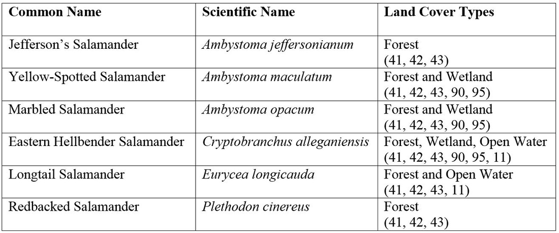
Table 1. Suitable land cover types by species.
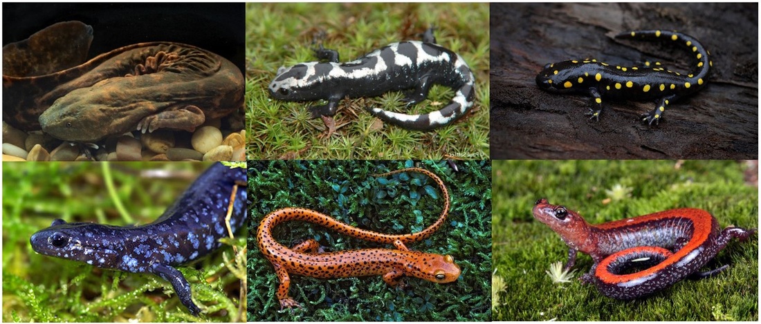
Figure 1. Images of each of the six Caudata species mapped in these analyses. From top-left to bottom-right: Eastern Hellbender, Marbled Salamander, Yellow-Spotted Salamander, Jefferson’s Salamander, Longtail Salamander, and Eastern Redbacked Salamander.
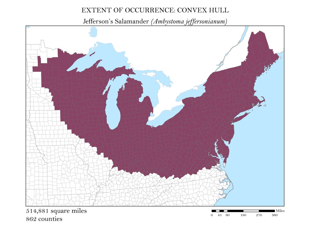
Figure 2a. Jefferson's Salamander: Extent of occurrence distribution map: convex hull.
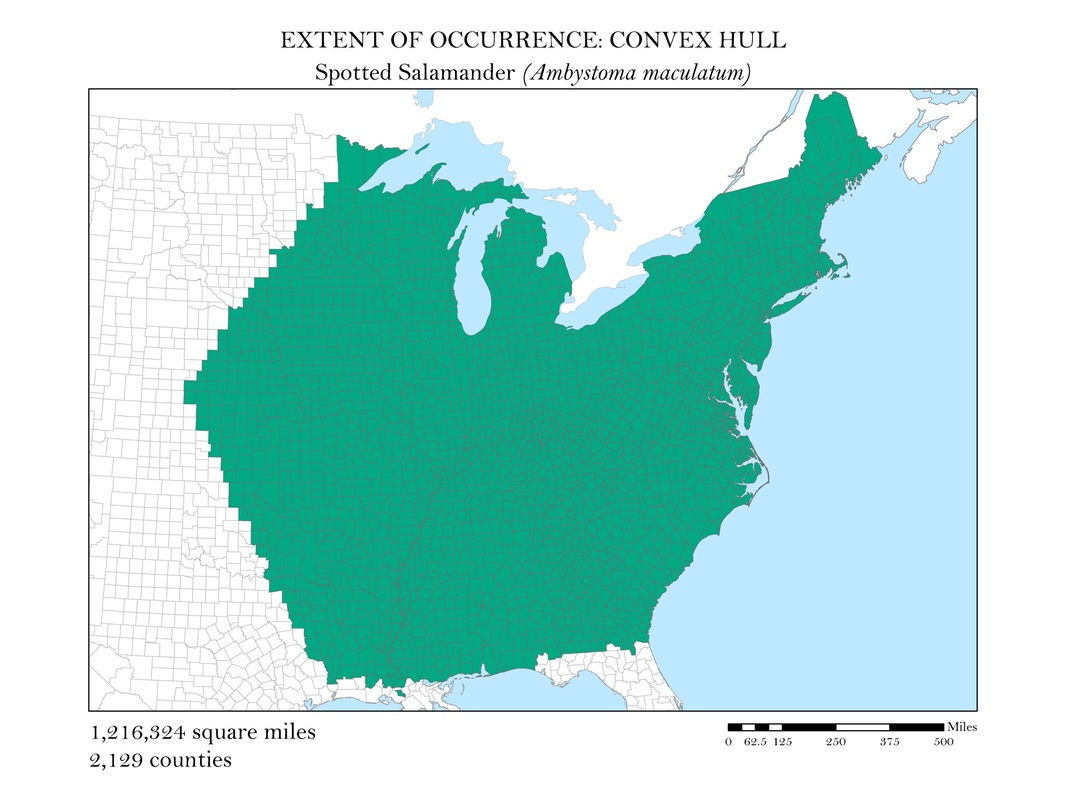
Figure 2b. Spotted Salamander: Extent of occurrence distribution map: convex hull.
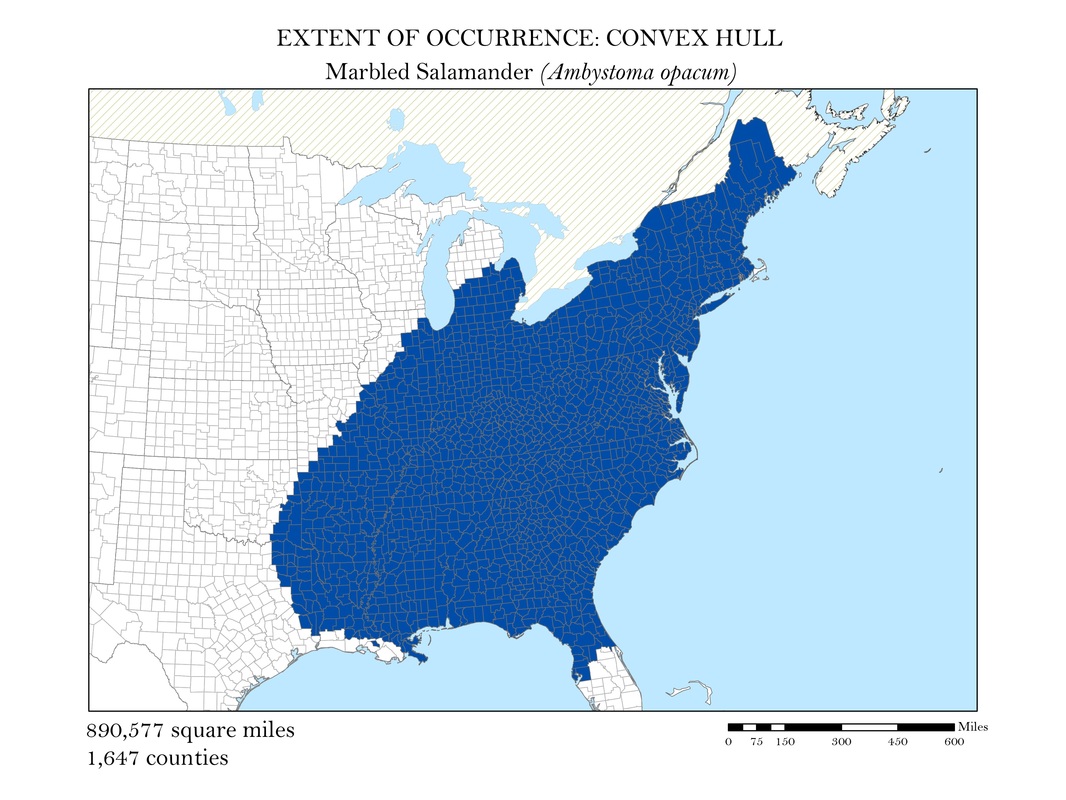
Figure 2c. Marbled Salamander: Extent of occurrence distribution map: convex hull.
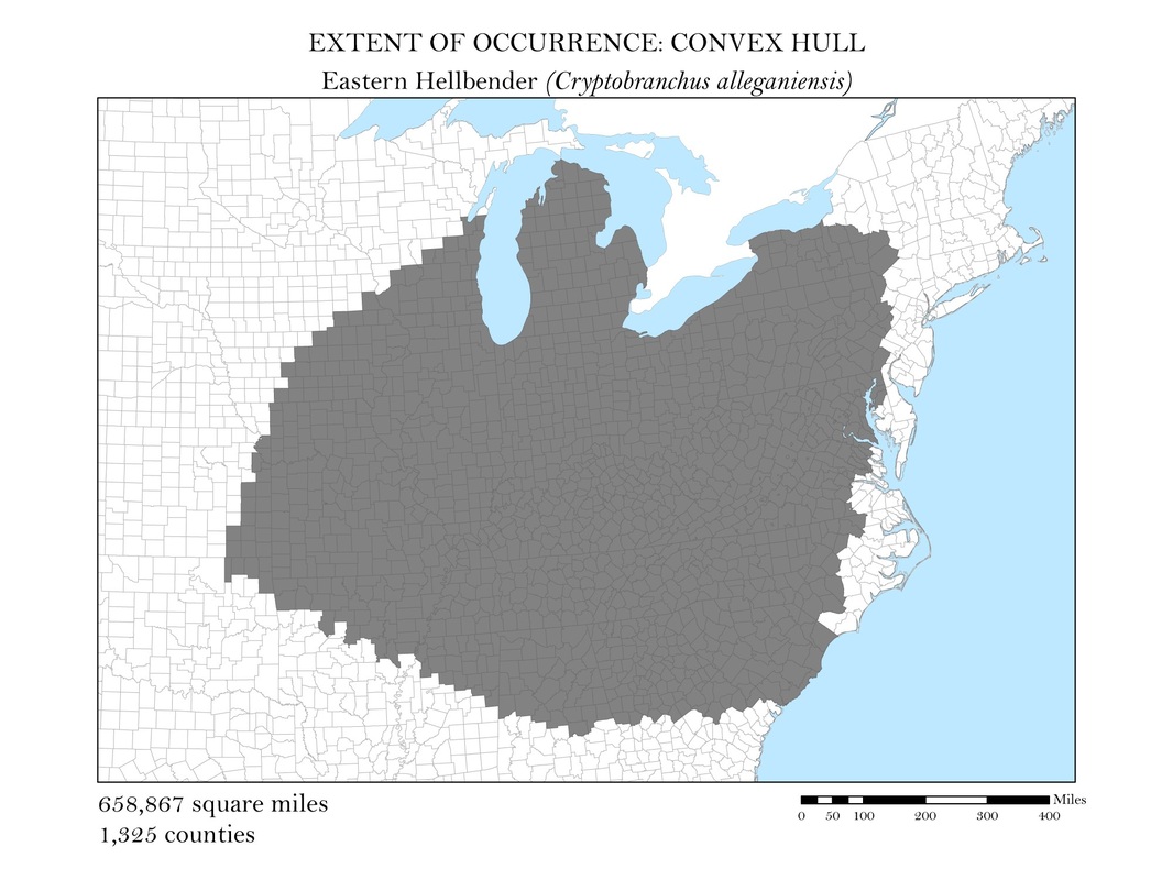
Figure 2d. Eastern Hellbender Salamander (Giant Salamander): Extent of occurrence distribution map: convex hull.
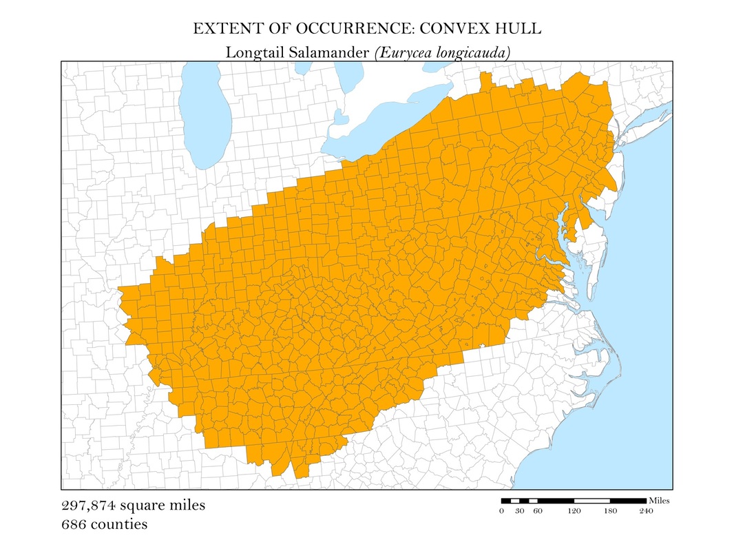
Figure 2e. Longtail Salamander: Extent of occurrence distribution map: convex hull.
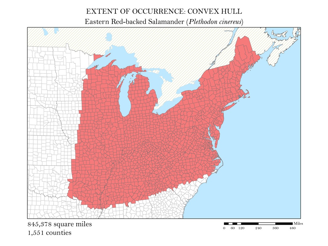
Figure 2f. Eastern Red-backed Salamander: Extent of occurrence distribution map: convex hull.
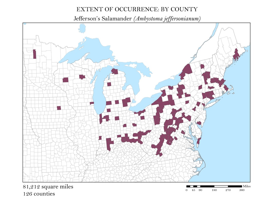
Figure 3a. Jefferson's Salamander: Extent of occurrence distribution map: by county.
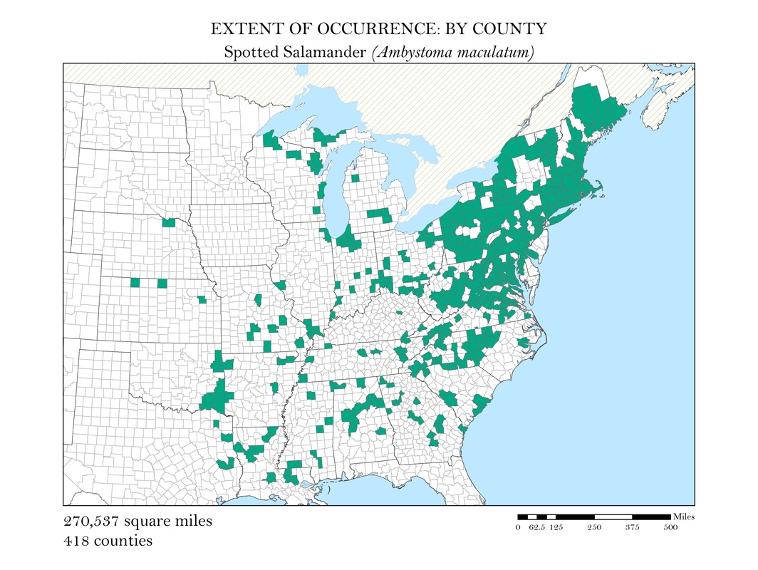
Figure 3b. Spotted Salamander: Extent of occurrence distribution map: by county.
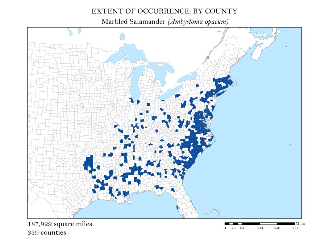
Figure 3c. Marbled Salamander: Extent of occurrence distribution map: by county.
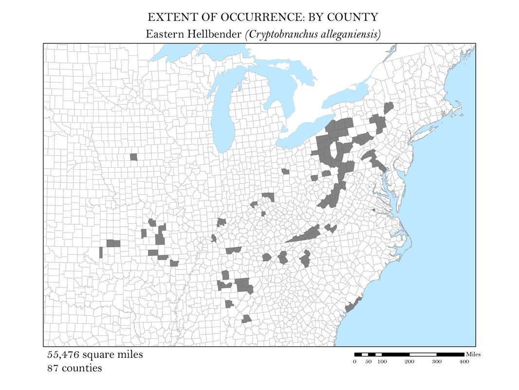
Figure 3d. Eastern Hellbender (Giant Salamander): Extent of occurrence distribution map: by county.
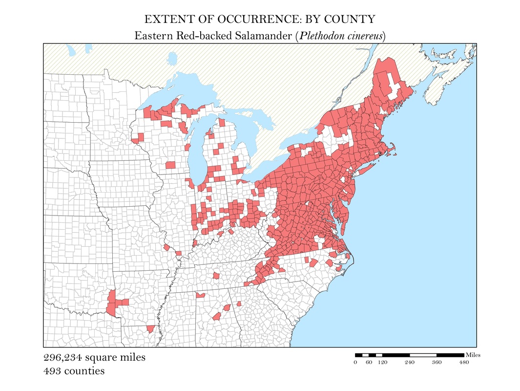
Figure 3e. Eastern Red-backed Salamander: Extent of occurrence distribution map: by county.
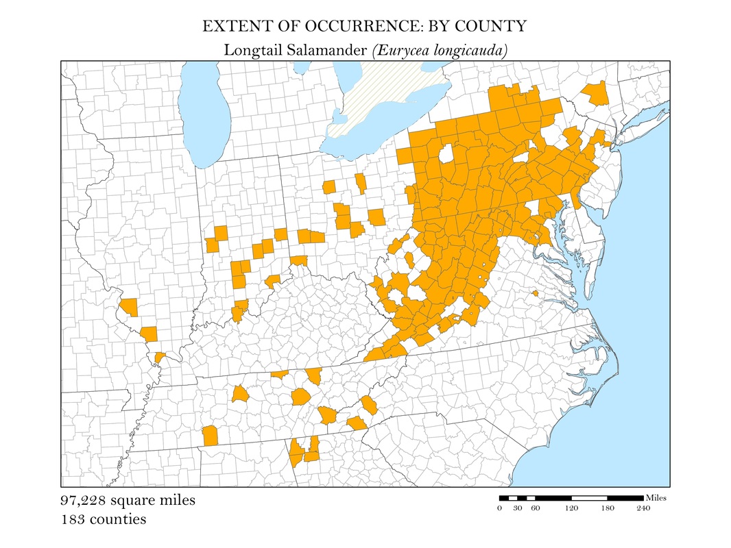
Figure 3f. Longtail Salamander: Extent of occurrence distribution map: by county.
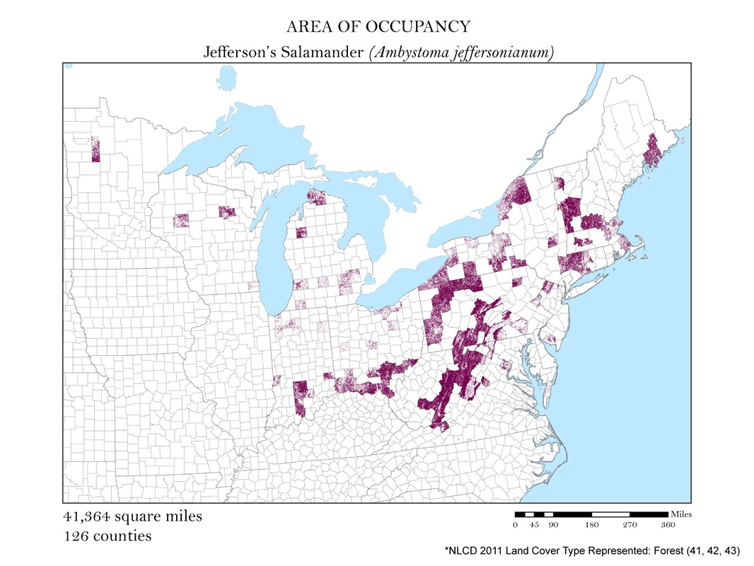
Figure 4a. Jefferson's Salamander: Area of occupancy distribution map.
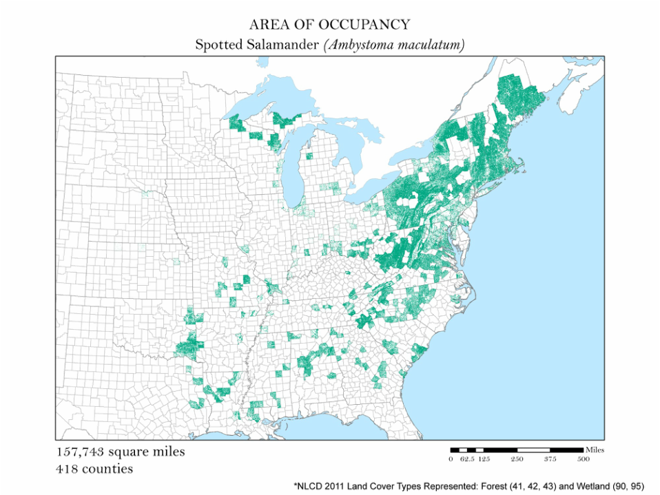
Figure 4b. Spotted Salamander: Area of occupancy distribution map.
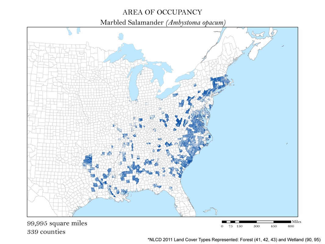
Figure 4c. Marbled Salamander: Area of occupancy distribution map.
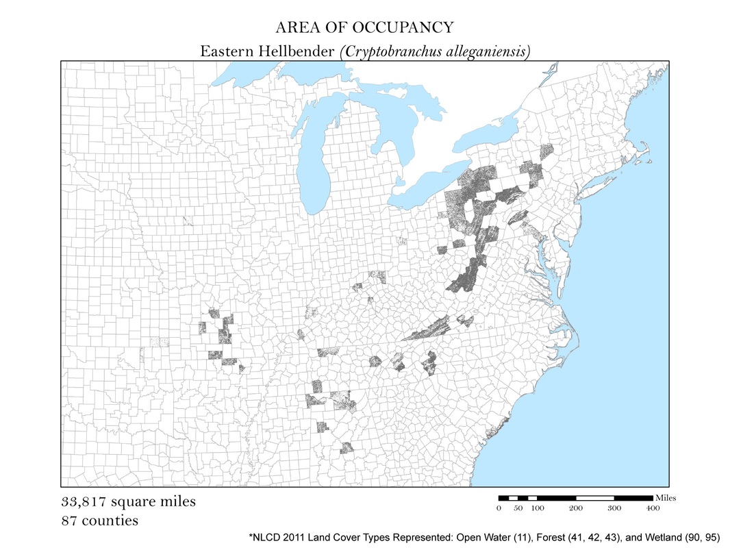
Figure 4d. Eastern Hellbender (Giant Salamander): Area of occupancy distribution map.
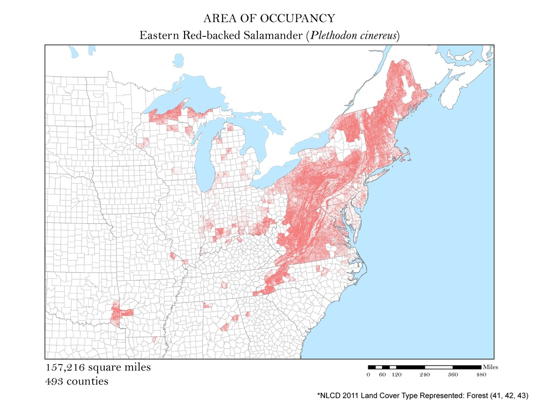
Figure 4a. Area of occupancy distribution map.
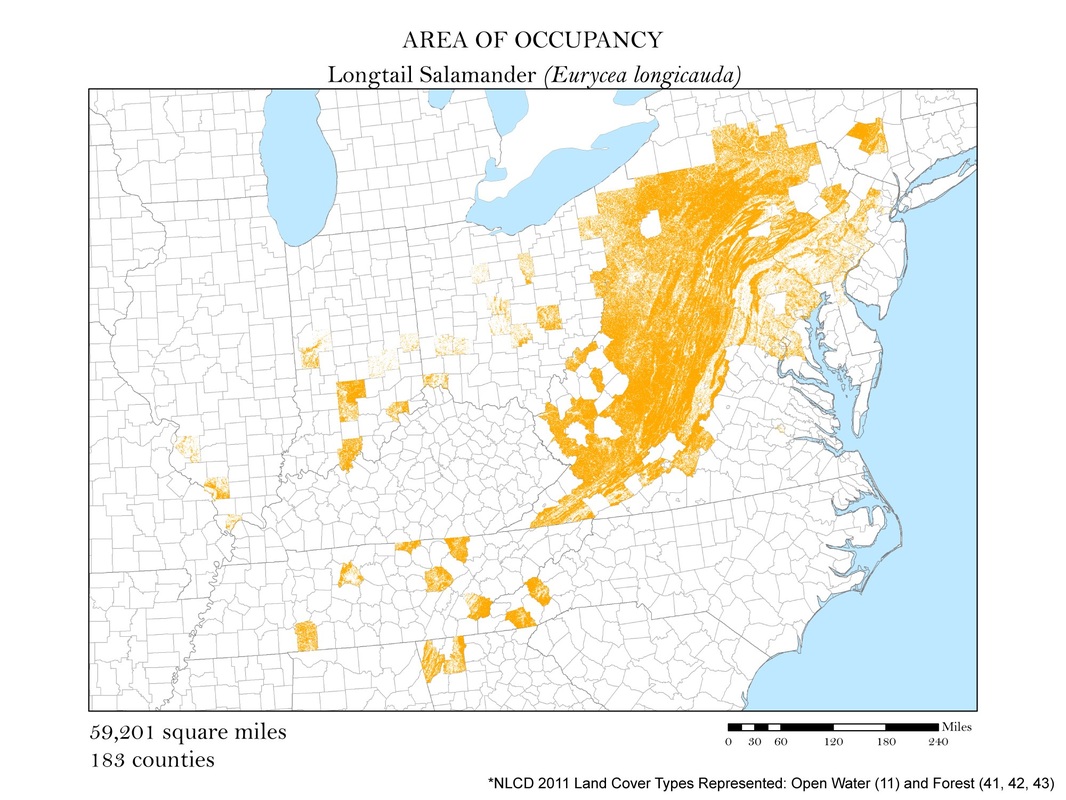
Figure 4f. Longtail Salamander: Area of occupancy distribution map.
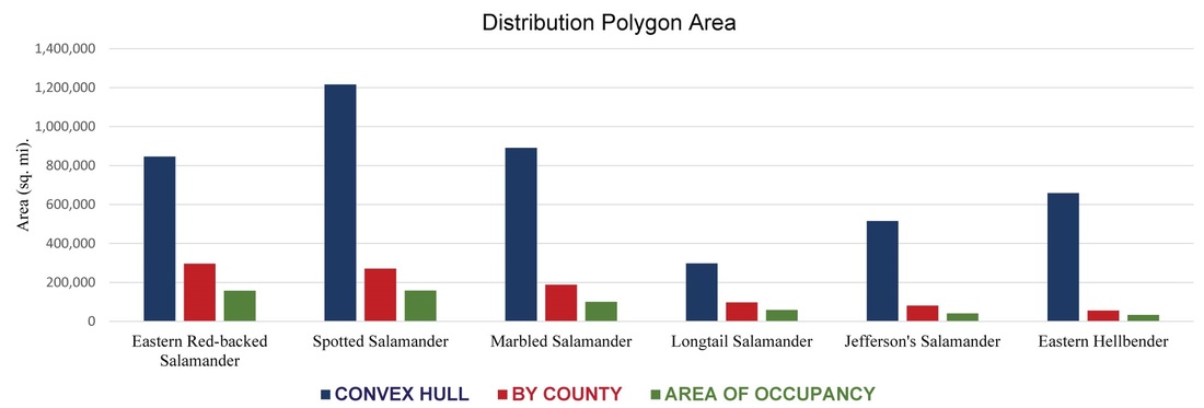
Figure 5. Calculations of area extrapolated from each of the three analyses.
Works Cited
Data:
(GBIF Data)
1. Academy of Natural Sciences: Herpetology
2. AMNH Herp Collection
3. California Academy of Sciences: CAS Herpetology (HERP)
4. Carnegie Museum of Natural History Herpetology Collection
5. Cincinnati Museum Center: CMC herpetology vouchers
6. Macaulay Library (ML).
7. Cornell Lab of Ornithology
8. Cornell University Museum of Vertebrates: CUMV Amphibian Collection (Arctos)
9. Cowan Tetrapod Collection at the University of British Columbia Beaty Biodiversity Museum (UBCBBM)
10. European Molecular Biology Laboratory (EMBL): Geographically tagged INSDC sequences
11. Herpetology Specimen Database of the Redpath Museum, McGill University.
12. iNaturalist.org: iNaturalist research-grade observations
13. INHS Herps Collection
14. institution collection catalog#
15. Laboratory for Environmental Biology, Centennial Museum, University of Texas at El Paso
16. Macaulay Library, www.macaulaylibrary.org
17. Macaulay Library/Cornell
18. Magaa Cota, G. E. 2004. Coleccian cientafica del Museo de Historia Natural Alfredo Dugas. Universidad de Guanajuato. Bases de datos SNIB2010-CONABIO. Proyecto No. V002. Macxico, D.F.
19. MHP Herp Collection
20. Milwaukee Public Museum
21. ML Audio 2081
22. ML Media-collection Catalog-number
23. Monty L. Bean Museum, Brigham Young University: Herpetology Collection
24. MSUM Ichthyology and Herpetology Collections
25. Musacum d'histoire naturelle de la Ville de Genave. Partial Amphibians Collection
26. Museum of Biological Diversity, The Ohio State University: Ohio State University Fish Division (OSUM)
27. Museum of Biological Diversity, The Ohio State University: Ohio State University Tetrapod Division - Amphibian Collection (OSUM)
28. Museum of Comparative Zoology, Harvard University: Museum of Comparative Zoology, Harvard University
29. Museum of Vertebrate Zoology (MVZ), University of California, Berkeley
30. National Museum of Natural History, Smithsonian Institution: NMNH occurrence DwC-A
31. Natural History Museum of Los Angeles County: LACM Vertebrate Collection
32. NatureServe Central Databases (accessed through GBIF data portal, http://data.gbif.org/datasets/resource/607, [DATE])
33. North Carolina Museum of Natural Sciences Herpetology Collection
34. PSM Collection
35. ROM Herp Collection
36. Royal Belgian Institute of Natural Sciences: RBINS collections
37. Royal Ontario Museum: Herpetology Collection - Royal Ontario Museum
38. Sam Noble Oklahoma Museum of Natural History: Amphibian Specimens
39. Sam Noble Oklahoma Museum of Natural History: Tissues Specimens
40. SBMNH Vertebrate Collection
41. SDNHM Herpetology Collection
42. Senckenberg: Collection Herpetologie - SNSD
43. Senckenberg: Collection Herpetology SMF
44. Spanish National Museum of Natural Sciences (CSIC): Museo Nacional de Ciencias Naturales, Madrid: MNCN Herpeto
45. Staatliches Museum far Naturkunde Stuttgart
46. Sutherland, Charles A
47. The Georgia Southern University - Savannah Science Museum Herpetology Collection
48. TNHC Herpetology Collection
49. UA Herps Collection
50. United States, New York, Tompkins, 3 km NE of Ithaca, Sapsucker Woods Pond
51. University of Alberta Museums: University of Alberta Museums, Amphibian and Reptile Collection
52. University of Colorado Museum of Natural History Amphibians and Reptiles Collection
53. University of Kansas Biodiversity Institute: KUBI Herpetology Collection
54. University of Tennessee - Chattanooga (UTC): (UTCA) University of Tennessee - Amphibians Collection
55. University of Washington Burke Museum Herpetology Collection
56. Varied sources. Individual references may be obtained from website (paleodb.org)
57. Wildlife Sightings - junponline (http://www.junponline.com)
58. Yale Peabody Museum, (c) 2009. Specimen data records available through distributed digital resources.
59. ZIN
Jin, S., Yang, L., Danielson, P., Homer, C., Fry, J., and Xian, G. 2013. A comprehensive change detection method for updating the National Land Cover Database to circa 2011. Remote Sensing of Environment, 132: 159 – 175.
U.S. Census Bureau, 2013. “cb_2013_us_county_5m.zip”. 5m = 1:5,000,000.
Images:
- http://chronicle.uchicago.edu/030403/salamanders.shtml
- http://ianadamsphotography.com/news/wp-content/gallery/wildlife/long-tailed-salamander-ashtabula-county-ohio.jpg
- http://images.nationalgeographic.com/wpf/media-live/photos/000/318/cache/fw-red-backed-salamander-1202424_31888_600x450.jpg
- http://voices.nationalgeographic.com/files/2013/08/Julie-Larsen-Maher-5881-Eastern-Hellbender-BZ-07-12-13.jpg
- http://www.virginiaherpetologicalsociety.com/amphibians/salamanders/marbled-salamander/Ambystoma%20opacum%20Pittsylvania%20Co.jpg
- http://www.wildlife.state.nh.us/Wildlife/Nongame/salamanders/salamander_images/bluespot4_Henk-Wallays.jpg
